Jacobi elliptic functions
In mathematics, the Jacobi elliptic functions are a set of basic elliptic functions, and auxiliary theta functions, that are of historical importance. Many of their features show up in important structures and have direct relevance to some applications (e.g. the equation of a pendulum—also see pendulum (mathematics)). They also have useful analogies to the functions of trigonometry, as indicated by the matching notation sn for sin. The Jacobi elliptic functions occur more often in practical problems than the Weierstrass elliptic functions. They were introduced by Carl Gustav Jakob Jacobi, around 1830.
Introduction
There are twelve Jacobian elliptic functions. Each of the twelve corresponds to an arrow drawn from one corner of a rectangle to another. The corners of the rectangle are labeled, by convention, s, c, d and n. The rectangle is understood to be lying on the complex plane, so that s is at the origin, c is at the point K on the real axis, d is at the point K + iK' and n is at point iK' on the imaginary axis. The numbers K and K' are called the quarter periods. The twelve Jacobian elliptic functions are then pq, where each of p and q is one of the letters s, c, d, n.
The Jacobian elliptic functions are then the unique doubly periodic, meromorphic functions satisfying the following three properties:
- There is a simple zero at the corner p, and a simple pole at the corner q.
- The step from p to q is equal to half the period of the function pq u; that is, the function pq u is periodic in the direction pq, with the period being twice the distance from p to q. The function pq u is also periodic in the other two directions, with a period such that the distance from p to one of the other corners is a quarter period.
- If the function pq u is expanded in terms of u at one of the corners, the leading term in the expansion has a coefficient of 1. In other words, the leading term of the expansion of pq u at the corner p is u; the leading term of the expansion at the corner q is 1/u, and the leading term of an expansion at the other two corners is 1.
More generally, there is no need to impose a rectangle; a parallelogram will do. However, if K and iK' are kept on the real and imaginary axis, respectively, then the Jacobi elliptic functions pq u will be real functions when u is real.
Notation
The elliptic functions can be given in a variety of notations, which can make the subject unnecessarily confusing. Elliptic functions are functions of two variables. The first variable might be given in terms of the amplitude φ, or more commonly, in terms of u given below. The second variable might be given in terms of the parameter m, or as the elliptic modulus k, where k2 = m, or in terms of the modular angle  , where
  . A more extensive review and definition of these alternatives, their complements, and the associated notation schemes are given in the articles on elliptic integrals and quarter period.
Definition as inverses of elliptic integrals
The above definition, in terms of the unique meromorphic functions satisfying certain properties, is quite abstract. There is a simpler, but completely equivalent definition, giving the elliptic functions as inverses of the incomplete elliptic integral of the first kind. This is perhaps the easiest definition to understand. Let
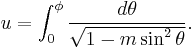
Then the elliptic function sn u is given by
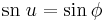
and cn u is given by

and
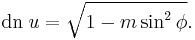
Here, the angle  is called the amplitude. On occasion, dn u = Δ(u) is called the delta amplitude. In the above, the value m is a free parameter, usually taken to be real, 0 ≤ m ≤ 1, and so the elliptic functions can be thought of as being given by two variables, the amplitude and the parameter m.
The remaining nine elliptic functions are easily built from the above three, and are given in a section below.
Note that when  , that u then equals the quarter period K.
Definition in terms of theta functions
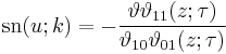
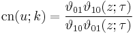
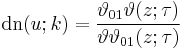
Equivalently, Jacobi elliptic functions can be defined in terms of his theta functions. If we abbreviate  as
as  , and
, and  respectively as
 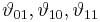 (the theta constants) then the elliptic modulus k is
 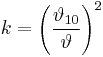 . If we set
  , we have
Since the Jacobi functions are defined in terms of the elliptic modulus  , we need to invert this and find τ in terms of k. We start from
  , the complementary modulus. As a function of τ it is
Let us first define
Then define the nome q as  and expand
  as a power series in the nome q, we obtain
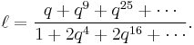
Reversion of series now gives

Since we may reduce to the case where the imaginary part of τ is greater than or equal to 1/2 sqrt(3), we can assume the absolute value of q is less than or equal to exp(-1/2 sqrt(3) π) ~ 0.0658; for values this small the above series converges very rapidly and easily allows us to find the appropriate value for q.
Minor functions
Reversing the order of the two letters of the function name results in the reciprocals of the three functions above:
![\begin{align}
\operatorname{ns}(u) & = \frac{1}{\operatorname{sn}(u)} \\[8pt]
\operatorname{nc}(u) & = \frac{1}{\operatorname{cn}(u)} \\[8pt]
\operatorname{nd}(u) & = \frac{1}{\operatorname{dn}(u)}
\end{align}](/2012-wikipedia_en_all_nopic_01_2012/I/4a4efaa95bb23c1ae539139b59ae2733.png)
Similarly, the ratios of the three primary functions correspond to the first letter of the numerator followed by the first letter of the denominator:
![\begin{align}
\operatorname{sc}(u) & = \frac{\operatorname{sn}(u)}{\operatorname{cn}(u)} \\[8pt]
\operatorname{sd}(u) & = \frac{\operatorname{sn}(u)}{\operatorname{dn}(u)} \\[8pt]
\operatorname{dc}(u) & = \frac{\operatorname{dn}(u)}{\operatorname{cn}(u)} \\[8pt]
\operatorname{ds}(u) & = \frac{\operatorname{dn}(u)}{\operatorname{sn}(u)} \\[8pt]
\operatorname{cs}(u) & = \frac{\operatorname{cn}(u)}{\operatorname{sn}(u)} \\[8pt]
\operatorname{cd}(u) & = \frac{\operatorname{cn}(u)}{\operatorname{dn}(u)}
\end{align}](/2012-wikipedia_en_all_nopic_01_2012/I/66d09824f09efec85118eaf52f2fc8ea.png)
More compactly, we have
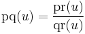
where each of p, q, and r is any of the letters s, c, d, n, with the understanding that ss = cc = dd = nn = 1.
(This notation is due to Gudermann and Glaisher and is not Jacobi's original notation.)
Addition theorems
The functions satisfy the two algebraic relations
From this we see that (cn, sn, dn) parametrizes an elliptic curve which is the intersection of the two quadrics defined by the above two equations. We now may define a group law for points on this curve by the addition formulas for the Jacobi functions
![\begin{align}
\operatorname{cn}(x%2By) & =
{\operatorname{cn}(x)\;\operatorname{cn}(y)
- \operatorname{sn}(x)\;\operatorname{sn}(y)\;\operatorname{dn}(x)\;\operatorname{dn}(y)
\over {1 - k^2 \;\operatorname{sn}^2 (x) \;\operatorname{sn}^2 (y)}}, \\[8pt]
\operatorname{sn}(x%2By) & =
{\operatorname{sn}(x)\;\operatorname{cn}(y)\;\operatorname{dn}(y) %2B
\operatorname{sn}(y)\;\operatorname{cn}(x)\;\operatorname{dn}(x)
\over {1 - k^2 \;\operatorname{sn}^2 (x)\; \operatorname{sn}^2 (y)}}, \\[8pt]
\operatorname{dn}(x%2By) & =
{\operatorname{dn}(x)\;\operatorname{dn}(y)
- k^2 \;\operatorname{sn}(x)\;\operatorname{sn}(y)\;\operatorname{cn}(x)\;\operatorname{cn}(y)
\over {1 - k^2 \;\operatorname{sn}^2 (x)\; \operatorname{sn}^2 (y)}}.
\end{align}](/2012-wikipedia_en_all_nopic_01_2012/I/33c6c9d310fe0e597caeda6831d3293e.png)
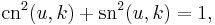
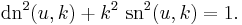
Relations between squares of the functions


where  and
and  .
.
Additional relations between squares can be obtained by noting that  and that
  where p, q, r are any of the letters s, c, d, n and ss = cc = dd = nn = 1.
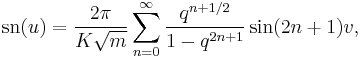
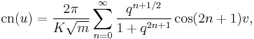
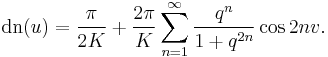
Expansion in terms of the nome
Let the nome be  and let the argument be
  . Then the functions have expansions as Lambert series
Jacobi elliptic functions as solutions of nonlinear ordinary differential equations
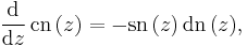
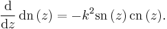
The derivatives of the three basic Jacobi elliptic functions are:
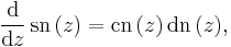
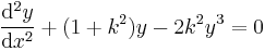
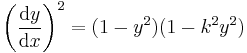
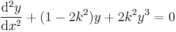
With the addition theorems above and for a given k with 0 < k < 1 they therefore are solutions to the following nonlinear ordinary differential equations:
 solves the differential equations
-
- and
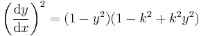
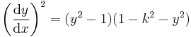
 solves the differential equations
-
- and
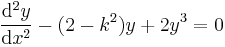
 solves the differential equations
-
- and
Map projection
The Peirce quincuncial projection is a map projection based on Jacobian elliptic functions.
See also
- Elliptic integral
- Elliptic curve
- Schwarz–Christoffel mapping
- Carlson symmetric form
- Weierstrass's elliptic functions
- Jacobi theta function
- Ramanujan theta function
References
- Abramowitz, Milton; Stegun, Irene A., eds. (1965), "Chapter 16", Handbook of Mathematical Functions with Formulas, Graphs, and Mathematical Tables, New York: Dover, pp. 569, ISBN 978-0486612720, MR0167642, http://www.math.sfu.ca/~cbm/aands/page_569.htm.
- N. I. Akhiezer, Elements of the Theory of Elliptic Functions, (1970) Moscow, translated into English as AMS Translations of Mathematical Monographs Volume 79 (1990) AMS, Rhode Island ISBN 0-8218-4532-2
- A. C. Dixon The elementary properties of the elliptic functions, with examples (Macmillan, 1894)
- Alfred George Greenhill The applications of elliptic functions (London, New York, Macmillan, 1892)
- H. Hancock Lectures on the theory of elliptic functions (New York, J. Wiley & sons, 1910)
- Reinhardt, William P.; Walker, Peter L. (2010), "Jacobian Elliptic Functions", in Olver, Frank W. J.; Lozier, Daniel M.; Boisvert, Ronald F. et al., NIST Handbook of Mathematical Functions, Cambridge University Press, ISBN 978-0521192255, MR2723248, http://dlmf.nist.gov/22
- E. T. Whittaker and G. N. Watson A Course of Modern Analysis, (1940, 1996) Cambridge University Press. ISBN 0-521-58807-3
- (French) P. Appell and E. Lacour Principes de la théorie des fonctions elliptiques et applications (Paris, Gauthier Villars, 1897)
- (French) G. H. Halphen Traité des fonctions elliptiques et de leurs applications (vol. 1) (Paris, Gauthier-Villars, 1886–1891)
- (French) G. H. Halphen Traité des fonctions elliptiques et de leurs applications (vol. 2) (Paris, Gauthier-Villars, 1886–1891)
- (French) G. H. Halphen Traité des fonctions elliptiques et de leurs applications (vol. 3) (Paris, Gauthier-Villars, 1886–1891)
- (French) J. Tannery and J. Molk Eléments de la théorie des fonctions elliptiques. Tome I, Introduction. Calcul différentiel. Ire partie (Paris : Gauthier-Villars et fils, 1893)
- (French) J. Tannery and J. Molk Eléments de la théorie des fonctions elliptiques. Tome II, Calcul différentiel. IIe partie (Paris : Gauthier-Villars et fils, 1893)
- (French) J. Tannery and J. Molk Eléments de la théorie des fonctions elliptiques. Tome III, Calcul intégral. Ire partie, Théorèmes généraux. Inversion (Paris : Gauthier-Villars et fils, 1893)
- (French) J. Tannery and J. Molk Eléments de la théorie des fonctions elliptiques. Tome IV, Calcul intégral. IIe partie, Applications (Paris : Gauthier-Villars et fils, 1893)
- (French) C. Briot and J. C. Bouquet Théorie des fonctions elliptiques ( Paris : Gauthier-Villars, 1875)